Project Echo: Can a Model Learn Animal Names From Sound?
A small-data audio classification study using mel spectrograms and MobileNetV2.
This study explores how wildlife recordings can be turned into mel spectrograms, classified with transfer learning, and checked on unseen videos to see whether the predicted animal name stays stable over time.
What I Studied
- 4 animal classes: Boar, Cane Toad, Foxes, and Tree Frogs.
- Mel spectrograms turned sound into a visual pattern the model could read.
- 5-second clips were used so the model learned from a consistent audio length.
- The final check used 3 unseen videos to compare label, confidence, and stability.
Why This Is Useful For Data Science And Business
Turn unstructured sound into structured data
Wildlife audio starts as raw sound. This pipeline converts it into features, class probabilities, labels, and model outputs that can be searched, summarized, and tracked.
Reduce manual review effort
A model can screen many recordings first, which helps people focus on the clips that are most likely to contain useful events.
Support monitoring and reporting
Predictions can feed simple summaries, alert logic, and trend analysis. That is the main business value of this kind of data science workflow.
How It Works
1. Audio preprocessing
Long recordings are clipped into consistent 5-second examples so the model trains on the same input length each time.
→
2. Mel spectrogram
Each clip becomes a time-frequency image. This makes rhythm and spectral shape easier to learn than a raw waveform.
→
3. MobileNetV2 classifier
A frozen MobileNetV2 backbone plus a small dense head classifies the spectrogram into one of four animal classes.
4. Window-level prediction
For longer media, the model predicts over sliding windows instead of one single pass.
→
5. Final label and confidence
Window predictions are averaged to produce the final label, confidence score, and a timeline of prediction behavior.
From First Run To Better Rerun
The rerun improved because the setup matched the dataset better. The gain came from cleaner small-data choices, not from making the model more complex.
Accuracy on the initial run
- Macro F1: 0.3214
- 7 training clips per class
- Larger trainable setup for a very small dataset
- Weak separation in the harder classes
Accuracy on the clean improved run
- Macro F1: 0.8667
- 9 training clips per class
- Frozen backbone with a smaller dense head
- Audio augmentation with noise and pitch variation
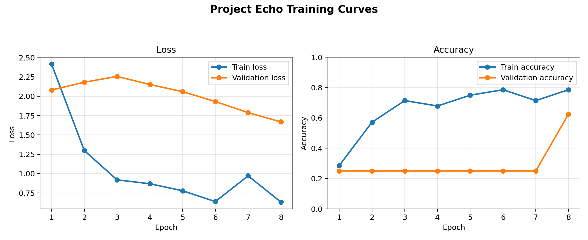
Baseline training curves
The first run was useful as a benchmark, but the learning pattern was not strong enough to produce reliable class separation.
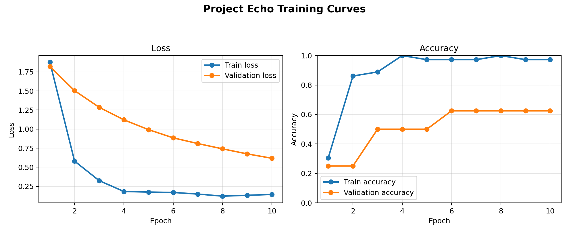
Improved training curves
The better rerun trained more cleanly and reached a much stronger result with a simpler small-data configuration.
Results
The strongest result was not just a better score. The rerun produced cleaner class separation, more stable predictions, and a more explainable path from sound to final label.
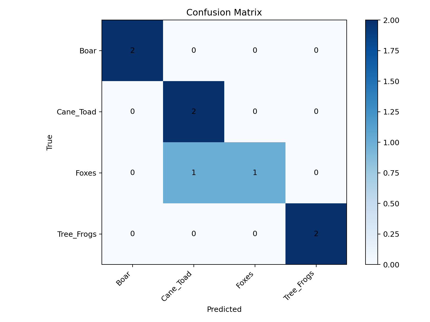
Confusion matrix
This figure shows that Boar and Tree Frogs are the clearest classes in the clean rerun. The main remaining confusion is still between Foxes and Cane Toad.
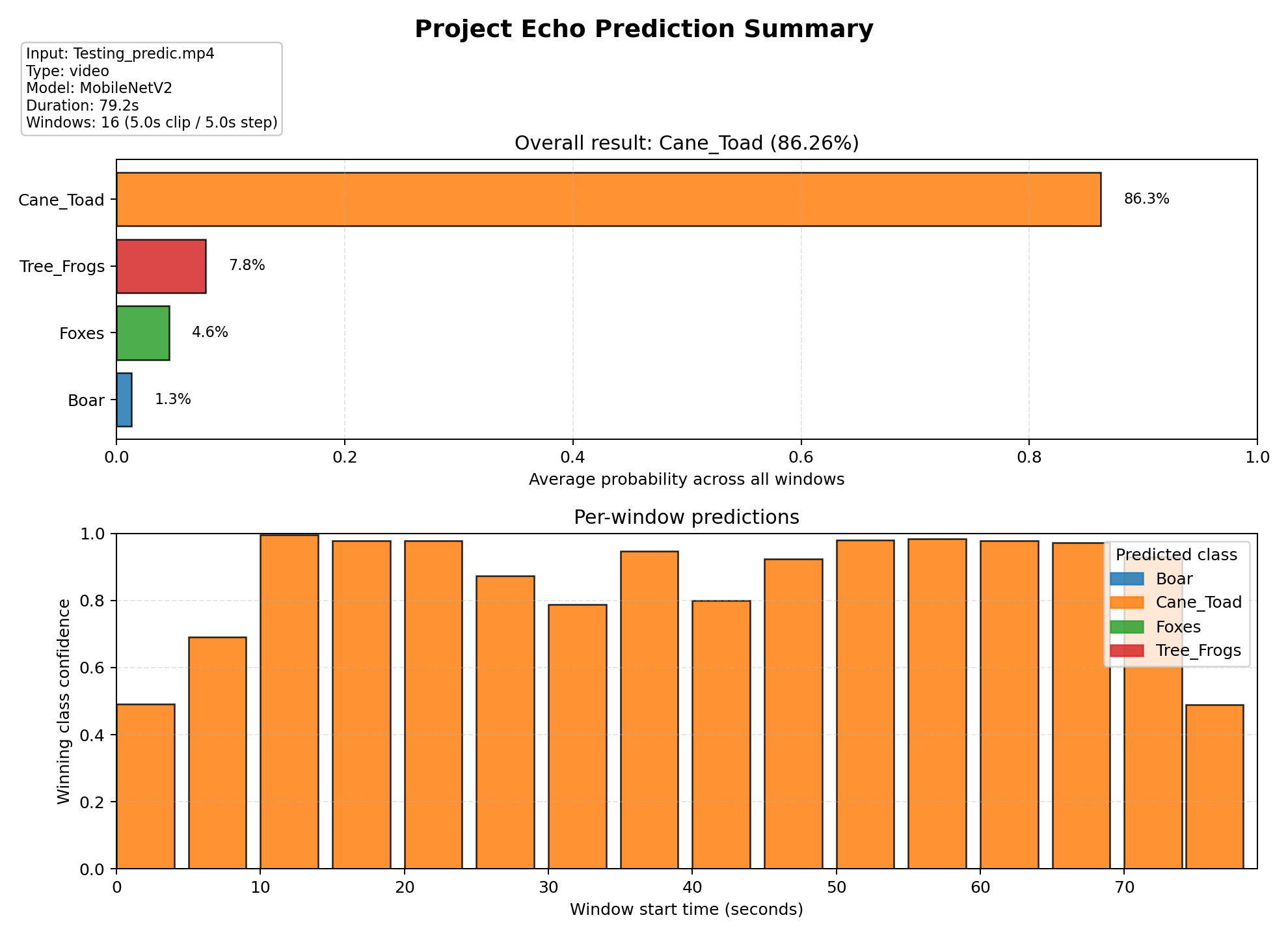
Prediction summary figure
This figure is useful because it shows both the final probabilities and the window-by-window behavior behind the final label. It makes the confidence story easier to understand than a single label alone.
The test split is still small at 8 clips total, so the improved result is promising but should be treated as an early study result rather than a final production-level claim.
Prediction On Unseen Videos
Strong Cane Toad example
Cane Toad · 86.26%
The clearest example. The model stays on Cane Toad across 16 windows, which suggests a repeated and stable acoustic pattern.
Mixed fox example
Foxes · 47.10%
A weaker prediction. Foxes wins overall, but Cane Toad and Boar compete in several windows, so this result is less certain.
Stronger fox example
Foxes · 58.88%
More confident than the previous fox sample, but still split with Cane Toad in multiple windows. This is the main class boundary that still needs work.
These video checks are useful because they show how confidence changes over time. A single final label can hide uncertainty, while window-level behavior shows whether the model is actually consistent.
What I Learned And Next Step
What I Learned
- Small datasets need a controlled setup. Simpler transfer learning worked better than a heavier trainable model.
- Mel spectrograms made the pipeline easier to understand because sound became a visible pattern.
- Video inference was important because it exposed which predictions were stable and which ones were only weakly dominant.
Next Step
- Add more source recordings per class so the model sees more recording conditions.
- Use source-level splits for a fairer measure of generalization.
- Focus on separating Foxes from Cane Toad more clearly, because that is the main remaining confusion.